Quantum ESPRESSO Hands-on Tutorial (Graphene)

B. Rebuilding Atomic Structures

This tutorial shows how to modify an existing crystal structure file to create a desired atomic configuration. Structures needed for calculations are not always available in the exact form we want. In many cases, we need to start from a crystal structure file obtained from a database such as Materials Project or from a previous calculation, and then modify the lattice parameters or atomic coordinates to create a structure suitable for our research. As a simple example, we will start from a graphene unit cell, create bilayer graphene, and adjust the relative position of one layer to construct AA and AB stacking. The goal of this tutorial is not simply to copy a particular set of coordinates, but to learn

how to understand an existing structure, calculate the required translation, and apply it to create the structure you want

Hexagonal Lattice Worksheet

Hexagonal lattice worksheet

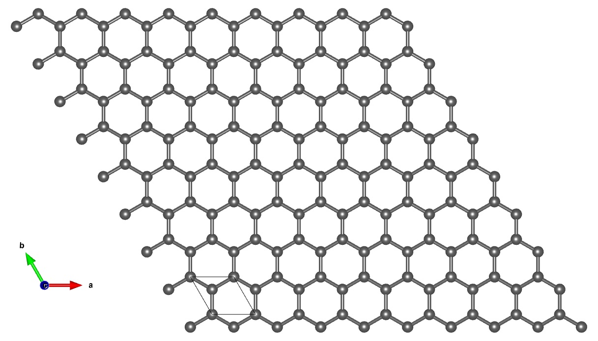
When calculating coordinates or translation vectors for hexagonal structures, I often use the worksheet below. I did not create this figure specifically for this tutorial. It is a reference I prepared and uploaded to my repository because I repeatedly use it when working with hexagonal cells. Hexagonal lattice worksheet

1. The $1:\sqrt{3}:2$ Triangle

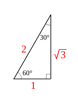
30°–60°–90° right triangle with the 1-sqrt(3)-2 side ratio

A hexagonal lattice can be divided into equilateral triangles. Dividing an equilateral triangle in half gives a $30^\circ$-$60^\circ$-$90^\circ$ right triangle, whose side lengths have the ratio $1:\sqrt{3}:2$. This is a simple geometric relationship, but it is the one I use most often when working with the worksheet.

This relationship is repeatedly useful when decomposing distances in a hexagonal structure into Cartesian $x$ and $y$ components. For graphene, the lattice constant $a$ and the nearest-neighbor C–C distance $d_{\mathrm{C-C}}$ are related by

$$a=\sqrt{3}d_{\mathrm{C-C}}$$

(and therefore $d_{\mathrm{C-C}} = \frac{a}{\sqrt{3}}$ ).

2. Starting Structure

We will use the following graphene unit cell as the starting structure.

vi hexagonal_cell.vasp

C
1.0
        2.4600000000         0.0000000000         0.0000000000
       -1.2300000000         2.1304224933         0.0000000000
        0.0000000000         0.0000000000        20.0000000000

C
2
Direct
        0.000000000          0.000000000          0.500000000
        0.333333333          0.666666667          0.500000000

The same structure in Cartesian coordinates is

C
1.0
        2.4600000000         0.0000000000         0.0000000000
       -1.2300000000         2.1304224933         0.0000000000
        0.0000000000         0.0000000000        20.0000000000

C
2
Cartesian
        0.000000000          0.000000000         10.000000000
        0.000000000          1.420281663         10.000000000

Direct coordinates $\mathbf{f}=(u,v,w)$ are converted to Cartesian coordinates using

$$\mathbf{r}=u\mathbf{a}_1+v\mathbf{a}_2+w\mathbf{a}_3.$$

The two in-plane lattice vectors are

$$\mathbf{a}_1 = (2.4600,\ 0,\ 0)$$

and

$$\mathbf{a}_2 = (-1.2300,\ 2.1304,\ 0)$$

respectively. The length of each vector is approximately

$$a=2.4600~\text{Å}$$

Using the $1:\sqrt{3}:2$ relationship introduced above,

$$d_{\mathrm{C-C}} = \frac{2.4600}{\sqrt{3}} \approx 1.4203~\text{Å} \approx 1.42~\text{Å}.$$

Thus, the nearest-neighbor C–C distance in this structure is approximately $1.42$ Å.

3. From Monolayer to Bilayer

The original file contains only a single graphene layer. To create a bilayer structure, we duplicate the two carbon atoms and place them at new $z$ coordinates. For example, in the current cell,

$$c=20~\text{Å}$$

and suppose we set the interlayer distance to

$$d=3.35~\text{Å}$$

The required layer separation in fractional coordinates is

$$\Delta z = \frac{3.35}{20} = 0.1675$$

If the two layers are placed symmetrically around the center of the cell, we can set

$$z_{\mathrm{lower}}=0.41625$$

and

$$z_{\mathrm{upper}}=0.58375$$

The actual interlayer distance is then

$$(0.58375-0.41625)\times20 = 3.35~\text{Å}$$

Here, we keep $c=20$ Å unchanged to make the connection between the original file and the calculation straightforward. In an actual isolated-bilayer DFT calculation, a larger vacuum thickness may be required.

AA Stacking

4. Constructing AA Stacking

In AA stacking, the carbon atoms in the upper and lower layers have the same in-plane positions. In other words, both sublattices overlap exactly when viewed from the top. Therefore, no in-plane translation is required, and the lattice vectors do not need to be changed. The AA-stacked structure can be constructed as follows.

AAstacking
1.0
        2.4600000000         0.0000000000         0.0000000000
       -1.2300000000         2.1304224933         0.0000000000
        0.0000000000         0.0000000000        20.0000000000
C
4
Direct
        0.000000000          0.000000000          0.416250000
        0.333333333          0.666666667          0.416250000
        0.000000000          0.000000000          0.583750000
        0.333333333          0.666666667          0.583750000

The same AA-stacked structure in Cartesian coordinates is

AAstacking
1.0
        2.4600000000         0.0000000000         0.0000000000
       -1.2300000000         2.1304224933         0.0000000000
        0.0000000000         0.0000000000        20.0000000000
C
4
Cartesian
        0.000000000          0.000000000          8.325000000
        0.000000000          1.420281663          8.325000000
        0.000000000          0.000000000         11.675000000
        0.000000000          1.420281663         11.675000000

The first two atoms belong to the lower layer, and the last two atoms belong to the upper layer. The key point is that the $x$ and $y$ coordinates are identical for the two layers. Also, because the number of atoms in the unit cell increases when going from a monolayer to a bilayer,

C
2

is changed to:

C
4

AB Stacking

5. What Changes in AB Stacking?

AB stacking is also commonly known as Bernal stacking. The difference between AA and AB stacking is not the size of the unit cell, but the relative in-plane position of the two graphene layers. In AB stacking, the entire upper layer is translated parallel to the graphene plane. After the translation,

one upper-layer carbon atom lies directly above a lower-layer carbon atom,
while the other upper-layer carbon atom lies above the center of a lower-layer graphene hexagon, that is, above a hollow site.

In other words,

$$\text{AA} \quad \xrightarrow{\text{in-plane translation of one layer}} \quad \text{AB}$$

To transform AA stacking into AB stacking, there is no need to change the in-plane lattice vectors or the unit-cell size.

6. Calculate the Translation by Hand

Now, let us calculate the required translation directly. The current lattice constant is

$$a=2.4600000000~\text{Å}$$

Using the $1:\sqrt{3}:2$ relationship, the nearest-neighbor C–C distance is

$$d_{\mathrm{C-C}} = \frac{a}{\sqrt{3}}$$

$$d_{\mathrm{C-C}} = \frac{2.4600}{\sqrt{3}} \approx 1.4203~\text{Å} \approx 1.42~\text{Å}.$$

With the current lattice-vector convention, we can use the following fractional translation:

$$\Delta\mathbf{f} = \left( \frac{1}{3},\frac{2}{3},0 \right).$$

In Cartesian coordinates, this translation can be written as

$$\Delta\mathbf{r} = \frac{1}{3}\mathbf{a}_1 + \frac{2}{3}\mathbf{a}_2$$

Therefore,

$$\Delta\mathbf{r} = \frac{1}{3} (2.4600,0,0) + \frac{2}{3} (-1.2300,2.1304,0).$$

The $x$ component is

$$\Delta x = \frac{2.4600}{3} - \frac{2(1.2300)}{3} \approx0$$

and the $y$ component is

$$\Delta y = \frac{2}{3}(2.13042) \approx 1.4203~\text{Å} \approx 1.42~\text{Å}$$

Therefore,

$$\boxed{ \Delta\mathbf{r} \approx (0,\ 1.4203,\ 0)~\text{Å} }$$

Interestingly, this value is identical to the C–C bond length obtained earlier using the $1:\sqrt{3}:2$ triangle. In other words, the hand-drawn hexagonal geometry and the calculation based on the actual lattice vectors give the same result.

7. Apply the Translation

Keep the fractional coordinates of the lower layer unchanged.

Lower layer

(0,        0,        0.41625)
(1/3,      2/3,      0.41625)

Apply the same translation vector to all atoms in the upper layer.

$$\Delta \mathbf{f} = \left( \frac{1}{3}, \frac{2}{3}, 0 \right).$$

Since the $z$ component is $0$, the height of the upper layer remains unchanged, and the layer is translated only in the $x$ and $y$ directions. The original fractional coordinate of the first upper-layer atom is

$$\left( 0, 0, 0.58375 \right)$$

Adding the translation vector gives

$$\left( 0, 0, 0.58375 \right) + \left( \frac{1}{3}, \frac{2}{3}, 0 \right) = \left( \frac{1}{3}, \frac{2}{3}, 0.58375 \right).$$

The original fractional coordinate of the second upper-layer atom is

$$\left( \frac{1}{3}, \frac{2}{3}, 0.58375 \right)$$

Applying the same translation gives

$$\left( \frac{1}{3}, \frac{2}{3}, 0.58375 \right) + \left( \frac{1}{3}, \frac{2}{3}, 0 \right) = \left( \frac{2}{3}, \frac{4}{3}, 0.58375 \right).$$

Because fractional coordinates follow periodic boundary conditions,

$$\frac{4}{3} \equiv \frac{1}{3} \pmod{1}.$$

Therefore,

$$\left( \frac{2}{3}, \frac{4}{3}, 0.58375 \right) \rightarrow \left( \frac{2}{3}, \frac{1}{3}, 0.58375 \right).$$

The final fractional coordinates of the upper layer in AB stacking are therefore

$$\left( \frac{1}{3}, \frac{2}{3}, 0.58375 \right)$$

and

$$\left( \frac{2}{3}, \frac{1}{3}, 0.58375 \right)$$

In other words, the lower layer remains unchanged, while the same in-plane translation is applied to the entire upper layer.

8. AB-Stacked Structure

The final AB-stacked structure is as follows.

ABstacking
1.0
        2.4600000000         0.0000000000         0.0000000000
       -1.2300000000         2.1304224933         0.0000000000
        0.0000000000         0.0000000000        20.0000000000
C
4
Direct
        0.000000000          0.000000000          0.416250000
        0.333333333          0.666666667          0.416250000
        0.333333333          0.666666667          0.583750000
        0.666666667          0.333333333          0.583750000

The same AB-stacked structure in Cartesian coordinates is

ABstacking
1.0
        2.4600000000         0.0000000000         0.0000000000
       -1.2300000000         2.1304224933         0.0000000000
        0.0000000000         0.0000000000        20.0000000000
C
4
Cartesian
        0.000000000          0.000000000          8.325000000
        0.000000000          1.420281663          8.325000000
        0.000000000          1.420281663         11.675000000
        1.230000000          0.710140831         11.675000000

The difference becomes clear when AA and AB stacking are compared directly.

AA

Lower:
(0,   0,   0.41625)
(1/3, 2/3, 0.41625)

Upper:
(0,   0,   0.58375)
(1/3, 2/3, 0.58375)

AB

Lower:
(0,   0,   0.41625)
(1/3, 2/3, 0.41625)

Upper:
(1/3, 2/3, 0.58375)
(2/3, 1/3, 0.58375)

The lattice vectors remain identical; only the relative position of the upper layer changes.

9. Check the Structure in VESTA

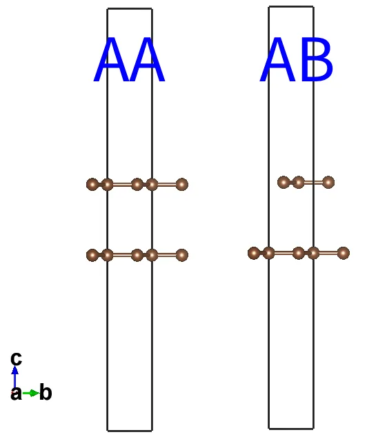
AA and AB stacking in bilayer graphene

Open the completed AA and AB files in VESTA and inspect the structures. When AA stacking is viewed along the $c$ axis, the carbon atoms in the upper and lower layers should overlap. In AB stacking, one upper-layer carbon atom should lie above a lower-layer carbon atom, while the other should lie above the center of a graphene hexagon. This step is more than just a visualization check. It allows us to verify that the coordinates we calculated actually produce the intended stacking configuration. The overall procedure can be summarized as follows.

Even when using an automated structure-generation tool, it is useful to understand how to perform these calculations. The desired structure may not always be generated automatically, and we may also need to independently verify whether the generated structure really has the geometry we intended.

Extending the Same Idea

AA/AB stacking in bilayer graphene is a very simple example, but the same approach can be extended directly to more complex structure construction. Examples include

multilayer stacking,
adsorbate–surface structures, …

Stacked Heterostructures

When stacking two different 2D materials, the questions are similar. For example, we need to decide whether a particular atom in the upper layer should be placed

above an atom in the lower layer,
above a bond center,
above a hexagonal hollow site.

To do this, a translation can be applied to the entire upper layer. However, when stacking different materials, additional factors must be considered compared with AA/AB graphene. For example,

supercell,
strain,
relative rotation,
interlayer distance, …

may need to be considered.

In other words, the process may involve more than a simple translation, but the basic idea remains the same.

Last updated on Oct 1, 2026

← A. Visualizing Atomic Structures