3. Graphene Projected Density of States
This tutorial continues from the graphene SCF calculation and calculates the projected density of states (PDOS) using an NSCF calculation followed by projwfc.x post-processing.
The important point is that the NSCF calculation reuses the converged ground-state data from the previous SCF calculation while sampling the Brillouin zone with a denser k-point mesh.
The resulting electronic states are then projected onto atomic orbitals, allowing us to examine the orbital character of the graphene electronic structure.
Create the working directory
Create a directory for the PDOS calculation and copy the required SCF input from the parent directory.
Prepare the NSCF input
Change the calculation type to nscf, use a denser k-point mesh, and include enough bands for the energy range of interest.
Run pw.x
Run the NSCF calculation to obtain the Kohn–Sham eigenvalues and wavefunctions on the dense k-point mesh.
Run projwfc.x
Project the electronic states onto atomic orbitals and generate the orbital-resolved density of states.
1. Create a PDOS-Calculation Directory
Start from the directory where the previous SCF calculation was prepared.
Create a separate directory for the PDOS calculation:
mkdir 99dos
cd 99dos
Copy the previous SCF input into the new directory:
cp ../1scf.in ./3nscf.in
cp -a ../out ./out
And then, :
.
├── 1scf.in
├── 1scf.out
├── 7501q.sh
├── out/              # original SCF data
└── 99pdos/
    └── out/          # copied data for NSCF/PDOS
The copied file will be used as the starting point for the NSCF input. This ensures that the lattice, atomic positions, pseudopotential, cutoffs, and other basic settings remain consistent with the SCF calculation.
For the SCF setup used in this tutorial:
2. Prepare the NSCF Input
Open the copied file:
vi 3nscf.in
The main changes from the SCF calculation are:
- change
calculation = 'scf'tocalculation = 'nscf' - point
outdirandpseudo_dirto the directories in the parent folder - optionally specify
nbnd - use a denser k-point mesh for Brillouin-zone sampling
An NSCF input based on the previous graphene SCF calculation can be written as:
&CONTROL
calculation = 'nscf'
etot_conv_thr = 2.0000d-05
forc_conv_thr = 1.0000d-04
outdir = './out/'
prefix = 'graphene'
pseudo_dir = '../pseudo/'
/

&SYSTEM
degauss = 0.01
ecutrho = 200
ecutwfc = 40
ibrav = 0
nat = 2
nbnd = 8
nosym = .false.
ntyp = 1
occupations = 'smearing'
smearing = 'mv'
/

&ELECTRONS
conv_thr = 4.000d-10
electron_maxstep = 80
mixing_beta = 0.4
/

ATOMIC_SPECIES
C 12.011 C.upf

ATOMIC_POSITIONS angstrom
C 0.0000000000 1.4202816622 0.0000000000
C 1.2300000000 0.7101408311 0.0000000000

K_POINTS automatic
36 36 1 0 0 0

CELL_PARAMETERS angstrom
2.4600000000 0.0000000000 0.0000000000
-1.2300000000 2.1304224933 0.0000000000
0.0000000000 0.0000000000 20.0000000000
Here, a $36 \times 36 \times 1$ k-point mesh is an example to sample the electronic states more densely than in the original SCF calculation.
3. Why Use an NSCF Calculation?
The SCF calculation determines the self-consistent ground-state electron density.
For the PDOS, however, we need the electronic eigenvalues and wavefunctions sampled over many k-points throughout the Brillouin zone.
An NSCF calculation reuses the converged potential from the SCF calculation and evaluates the electronic states on a new k-point mesh without repeating the full self-consistency cycle.
Why not use the SCF k-point mesh directly?
The SCF k-point mesh is chosen primarily to converge the ground-state electron density and total energy.
Using a denser NSCF mesh improves the sampling without repeating the full self-consistent calculation.
4. K-point Sampling for the PDOS
In the previous SCF calculation, the Brillouin zone was sampled using:
K_POINTS automatic
12 12 1 0 0 0
For the NSCF calculation, this is increased to:
K_POINTS automatic
36 36 1 0 0 0
The denser in-plane mesh provides more electronic states for constructing the projected density of states.
Because graphene is two-dimensional and the third lattice direction contains vacuum, only one k-point is used along the $z$-direction.
5. Run the NSCF Calculation
Local execution
Run the NSCF calculation using:
pw.x -in 3nscf.in > 3nscf.out
For an MPI calculation:
mpirun -np 4 pw.x -in 3nscf.in > 3nscf.out
HPC job submission
On a SLURM-based cluster, the calculation can be submitted through the same job-submission workflow used for the previous calculations. qe_job_submit.sh on GitHub ↗
sbatch qe_job_submit.sh
6. Check the NSCF Output
After the calculation finishes, inspect the end of the output file:
tail -50 3nscf.out
You can also check that the job finished normally:
grep "JOB DONE" 3nscf.out
At this stage, pw.x has calculated the electronic eigenvalues and wavefunctions on the dense k-point mesh.
The next step is to project these electronic states onto atomic orbitals using projwfc.x.
7. Prepare the projwfc.x Input
Create an input file named:
3nscf.2pdos.in
with:
&PROJWFC
prefix = 'graphene'
outdir = './out/'
filpdos = 'graphene'
Emin = -10.0
Emax = 10.0
DeltaE = 0.01
/
The main parameters are:
prefixidentifies the QE calculation to be processed.outdirpoints to the directory containing the NSCF data.filpdosdefines the prefix used for the PDOS output files.EminandEmaxdefine the energy range.DeltaEdefines the energy spacing of the output.
The energy range shown here is only an example.
Choose Emin and Emax according to the electronic states you want to examine.
8. Run projwfc.x
Run the PDOS post-processing calculation:
projwfc.x -in 3nscf.2pdos.in > 3nscf.2pdos.out
projwfc.x projects the calculated Kohn–Sham states onto atomic orbitals and generates orbital-resolved density-of-states files.
The generated filenames depend on the atomic species and orbital character included in the pseudopotential.
For carbon, the output typically contains contributions associated with the $s$ and $p$ orbitals.
projwfc.x does not perform a new electronic-structure calculation.
It post-processes the wavefunctions obtained from the preceding pw.x calculation and resolves them into atomic-orbital contributions.
9. Understanding the PDOS
The projected density of states allows us to examine which atomic orbitals contribute to the electronic states at a given energy.
For graphene, the most relevant carbon orbitals are:
C 2s
C 2p_x
C 2p_y
C 2p_z
The in-plane $s$, $p_x$, and $p_y$ orbitals mainly contribute to the $\sigma$-bonding network.
The out-of-plane $p_z$ orbitals form the $\pi$ and $\pi^\ast$ states that dominate the electronic structure near the Dirac point.
Why is the p_z orbital important in graphene?
Each carbon atom in graphene forms strong in-plane $\sigma$ bonds using orbitals lying primarily in the graphene plane.
The remaining $p_z$ orbital extends perpendicular to the plane and overlaps with neighboring $p_z$ orbitals.
These states form the $\pi$ and $\pi^\ast$ bands that meet near the $K$ and $K'$ points and produce graphene’s characteristic Dirac-cone electronic structure.
10. Inspect the PDOS Files
After running projwfc.x, check the generated files:
ls
You should see several files associated with the total and orbital-projected density of states.
The exact filenames depend on the orbital labels written by projwfc.x, but they typically contain information about:
- the atom index,
- the atomic species,
- the angular-momentum channel,
- and the corresponding projected DOS.
These files can be combined or plotted separately depending on the quantity of interest.
For example, the carbon $p_z$ contribution can be compared with the total $p$-orbital contribution to identify the states associated with the graphene $\pi$ bands.
11. Energy Reference
For plotting, it is often useful to shift the energy axis relative to the Fermi energy:
$$ E - E_F. $$With this convention, the Fermi level is located at:
$$ E - E_F = 0. $$This makes it easier to compare the PDOS with the previously calculated band structure.
Near the Dirac point, the density of states approaches zero, while the electronic states in this energy range are dominated by the carbon $p_z$ orbitals.
12. Workflow Summary
The complete PDOS workflow is:
SCF (pw.x)
 ↓
Converged ground-state density
 ↓
NSCF calculation (pw.x) on a dense k-point mesh
 ↓
Electronic eigenvalues and wavefunctions
 ↓
projwfc.x
 ↓
Orbital-projected density of states
 ↓
Plot
The PDOS provides information that cannot be obtained from the band structure alone.
The band structure shows how the electronic energies vary with crystal momentum, while the PDOS reveals the atomic-orbital character of those states.
For graphene, the most important result is the strong $p_z$ character of the electronic states near the Dirac point, corresponding to the $\pi$ and $\pi^\ast$ bands.
13. Plot the Band Structure with PDOS
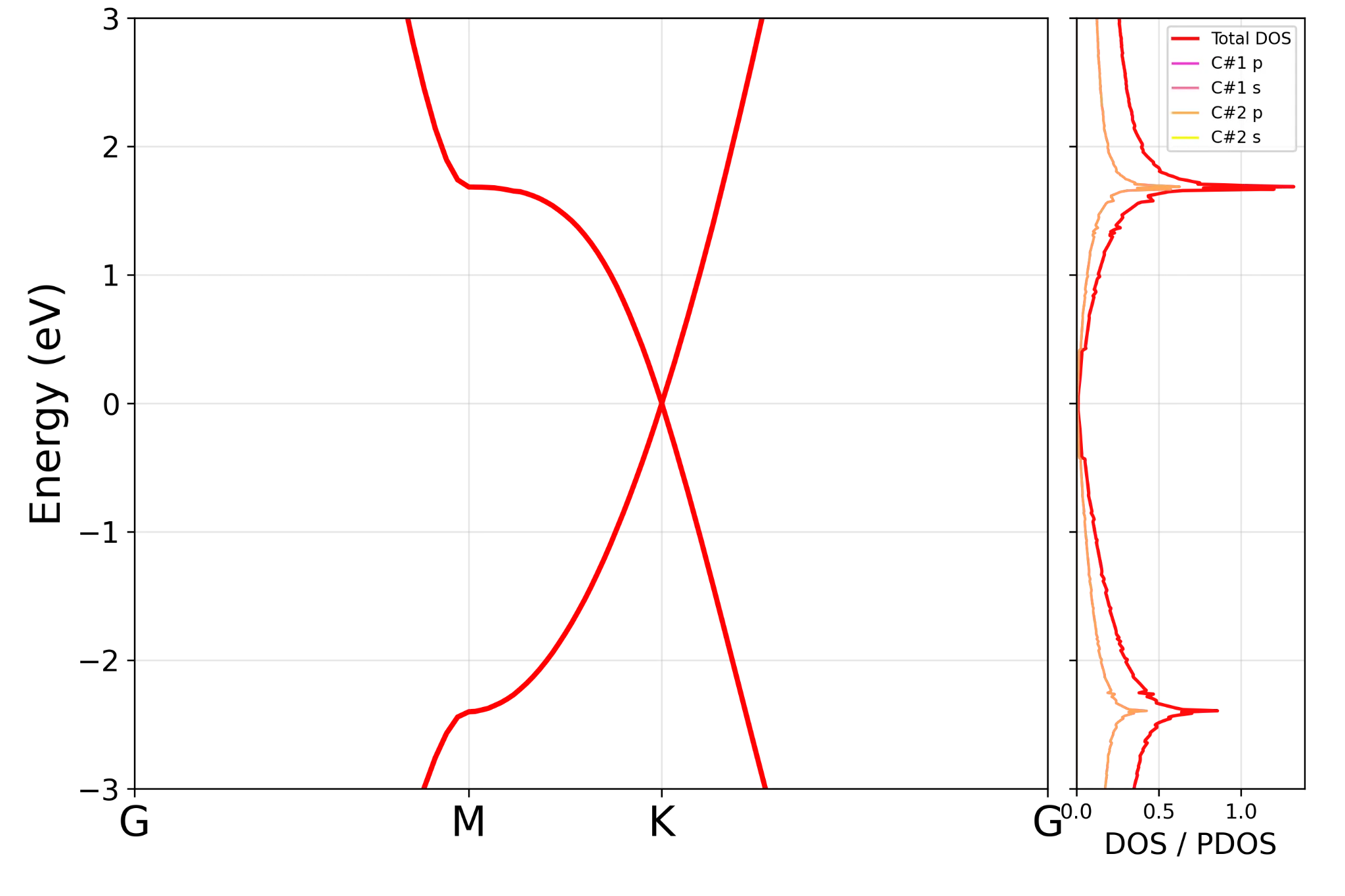
After completing the band-structure and PDOS calculations in the same directory, the band dispersion and projected density of states can be plotted together using qebands.py on GitHub ↗.
At this stage, the directory structure can look like:
.
├── 1scf.in
├── 1scf.out
├── 7501q.sh
├── out/              # original SCF data
└── 99pdos/
    ├── out/                              # copied data for NSCF/PDOS/band calculations
    ├── 3nscf.in
    ├── 3nscf.out
    ├── 3nscf.2pdos.in
    ├── 3nscf.2pdos.out
    ├── 99band.1pw.in
    ├── 99band.1pw.out
    ├── 99band.2pp.in
    ├── 99band.2pp.out
    ├── band.dat.gnu
    ├── graphene.pdos_tot
    ├── graphene.pdos_atm#1(C)_wfc#1(s)
    ├── graphene.pdos_atm#1(C)_wfc#2(p)
    ├── graphene.pdos_atm#2(C)_wfc#1(s)
    ├── graphene.pdos_atm#2(C)_wfc#2(p)
    └── qebands.py
Here, 99band.1pw.in and 99band.2pp.in were used in the previous tutorial, while 3nscf.in and 3nscf.2pdos.in are used in this tutorial. When the PDOS files and bands structure outputs are present in the same directory, the script adds the total DOS and orbital-resolved PDOS as a panel next to the band structure. This makes it possible to directly compare the band dispersion with the orbital character of the electronic states.
The plotting script automatically searches the same directory for the Fermi energy, high-symmetry-point information, and available *.pdos_tot and *.pdos_atm#* files. Furthermore, the energies are shifted relative to the Fermi level, so the plotted energy is $
E - E_F.$
Run:
python qebands.py
The script also writes the plotted data and saves the figure as image files. A representative result is shown below.