B. Rebuilding Atomic Structures

이 글에서는 기존의 crystal structure file을 활용하여 원하는 atomic configuration으로 수정하는 방법을 살펴본다. 왜냐하면 계산에 필요한 구조가 항상 원하는 형태로 제공되는 것은 아니기 때문이다. Materials Project와 같은 데이터베이스나 기존 계산에서 얻은 crystal structure file을 출발점으로 사용하고, lattice parameters 또는 atomic coordinates를 수정하여 연구 목적에 맞는 구조를 만들어야 하는 경우가 많다. 간단한 예제로 graphene unit cell을 사용하여 bilayer graphene을 만들고, 한 층의 상대적인 위치를 조절하여 AA 및 AB stacking을 구성한다. 이 튜토리얼의 목표는 특정 좌표를 그대로 따라 쓰는 것이 아니라,

기존 구조를 이해하고, 필요한 translation을 계산하고, 그것을 내가 원하는 구조에 적용하는 방법 을 익히는 것이다.

Hexagonal Lattice Worksheet

Hexagonal structure의 좌표나 translation vector를 계산할 때 나는 아래 worksheet를 자주 사용한다. 이 그림은 이 튜토리얼을 위해 새로 만든 것이 아니라, 실제로 hexagonal cell을 다룰 때 반복해서 사용하기 때문에 개인적으로 정리하여 repository에 올려 둔 자료이다. Hexagonal lattice worksheet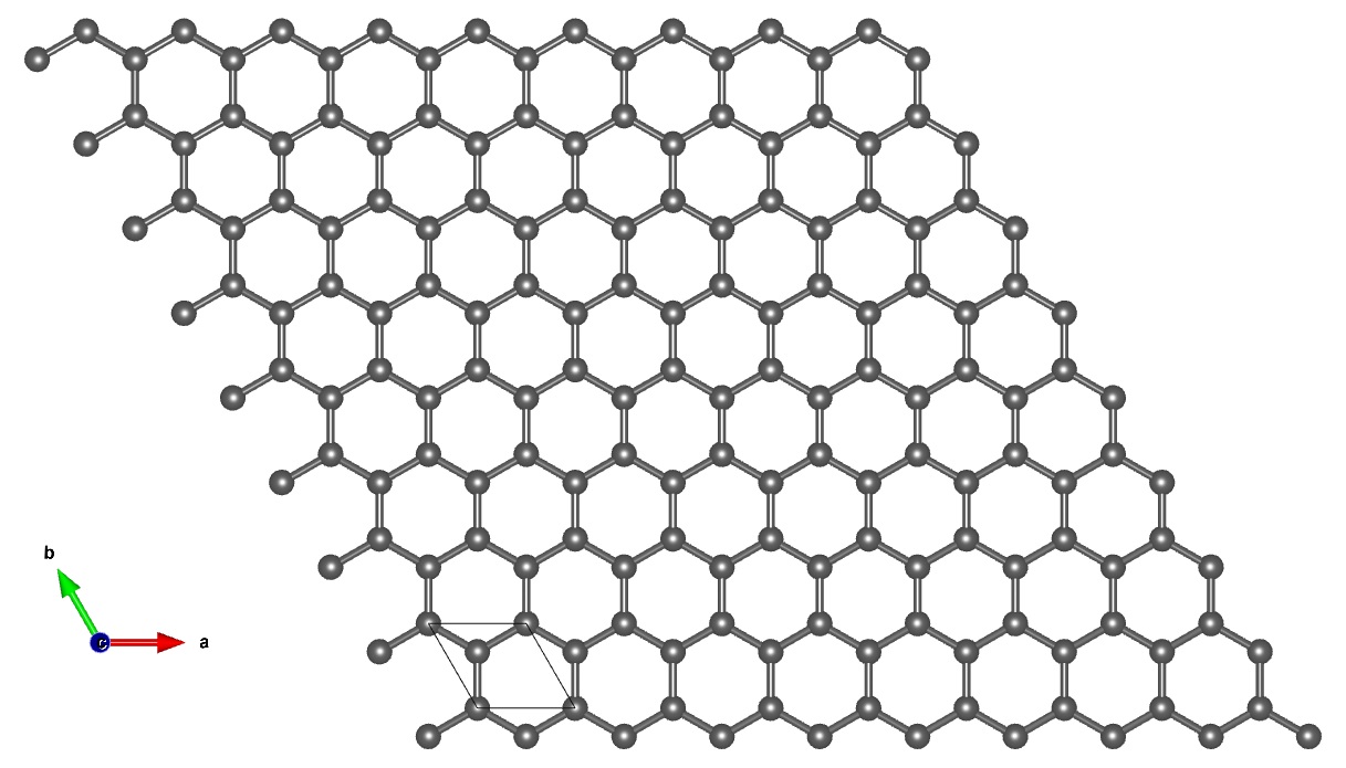

1. The $1:\sqrt{3}:2$ Triangle

Hexagonal lattice는 정삼각형으로 나눌 수 있다. 정삼각형을 반으로 나누면 $30^\circ$-$60^\circ$-$90^\circ$ 직각삼각형이 되고, 변의 길이는 $1:\sqrt{3}:2$ 의 비를 가진다. 당연한 내용이지만 worksheet에서 계산할 때 가장 많이 쓰는 내용이다.

30°–60°–90° right triangle with the 1-sqrt(3)-2 side ratio

이 관계는 hexagonal structure에서 거리를 Cartesian $x$ 및 $y$ 성분으로 분해할 때 반복해서 사용된다. Graphene에서는 lattice constant $a$와 nearest-neighbor C–C distance $d_{\mathrm{C-C}}$ 사이에

$$a=\sqrt{3}d_{\mathrm{C-C}}$$

의 관계가 있다(따라서 $d_{\mathrm{C-C}} = \frac{a}{\sqrt{3}}$ ).

2. Starting Structure

다음 graphene unit cell을 출발점으로 사용한다.

vi hexagonal_cell.vasp

C
1.0
        2.4410462379         0.0000000000         0.0000000000
       -1.2205234005         2.1140078914         0.0000000000
        0.0000000000         0.0000000000        20.0000000000

C
2
Direct
        0.000000000          0.000000000          0.500000000
        0.333333333          0.666666667          0.500000000

두 in-plane lattice vectors는

$$\mathbf{a}_1 = (2.4410462379,\ 0,\ 0)$$

및

$$\mathbf{a}_2 = (-1.2205234005,\ 2.1140078914,\ 0)$$

이다. 두 벡터의 길이는 약

$$a=2.4410~\text{Å}$$

이다. 앞에서 본 $1:\sqrt{3}:2$ 관계를 사용하면,

$$d_{\mathrm{C-C}} = \frac{2.4410}{\sqrt{3}} \approx 1.4093~\text{Å}.$$

즉, 이 구조에서 nearest-neighbor C–C distance는 약 $1.409$ Å이다.

3. From Monolayer to Bilayer

원래 파일에는 graphene layer가 하나만 존재한다. Bilayer structure를 만들기 위해 두 carbon atoms를 복제하고 새로운 $z$ coordinate에 배치한다. 예를 들어 현재 cell에서

$$c=20~\text{Å}$$

이고, interlayer distance를

$$d=3.35~\text{Å}$$

로 설정한다고 하자. Fractional coordinate에서 필요한 layer separation은

$$\Delta z = \frac{3.35}{20} = 0.1675$$

이다. 두 층을 cell center를 기준으로 대칭적으로 배치하면

$$z_{\mathrm{lower}}=0.41625$$

및

$$z_{\mathrm{upper}}=0.58375$$

로 둘 수 있다. 그러면 실제 층간 거리는

$$(0.58375-0.41625)\times20 = 3.35~\text{Å}$$

가 된다.

여기서는 원래 파일과 계산을 간단히 연결하기 위해 $c=20$ Å를 그대로 사용한다. 실제 isolated bilayer DFT 계산에서는 더 큰 vacuum thickness가 필요할 수 있다.

AA Stacking

4. Constructing AA Stacking

AA stacking에서는 upper layer와 lower layer의 carbon atoms가 동일한 in-plane position을 가진다. 즉 top view에서 두 sublattice가 모두 정확히 겹쳐 보인다. 따라서 in-plane translation은 필요하지 않으며, lattice vectors도 바꿀 필요가 없다. AA-stacked structure는 다음과 같이 만들 수 있다.

C
1.0
        2.4410462379         0.0000000000         0.0000000000
       -1.2205234005         2.1140078914         0.0000000000
        0.0000000000         0.0000000000        20.0000000000

C
4
Direct
        0.000000000          0.000000000          0.416250000
        0.333333333          0.666666667          0.416250000
        0.000000000          0.000000000          0.583750000
        0.333333333          0.666666667          0.583750000

앞의 두 atoms는 lower layer에 속하고, 뒤의 두 atoms는 upper layer에 속한다. 핵심은 두 층의 $x$ 및 $y$ coordinates가 동일하다는 점이다. 또한, monolayer에서 bilayer로 한 unit cell 안의 원자가 늘어났기 때문에

C
2

이 부분이 아래와 같이 바뀌었다:

C
4

AB Stacking

5. What Changes in AB Stacking?

AB stacking은 흔히 Bernal stacking이라고도 한다. AA와 AB의 차이는 unit-cell 크기가 아니라 두 graphene layer 사이의 상대적인 in-plane position이다. AB stacking에서는 upper layer 전체를 graphene plane과 평행한 방향으로 이동시킨다. 이동 후에는

upper-layer carbon 하나가 lower-layer carbon 바로 위에 위치하고,
다른 upper-layer carbon은 lower-layer graphene hexagon의 중심, 즉 hollow site 위에 위치한다. 즉,

$$\text{AA} \quad \xrightarrow{\text{in-plane translation of one layer}} \quad \text{AB}$$

이다. AA에서 AB로 바꾸기 위해 in-plane lattice vectors나 unit-cell size를 바꿀 필요는 없다.

6. Calculate the Translation by Hand

이제 필요한 translation을 직접 계산해 보자. 현재 lattice constant는

$$a=2.4410462379~\text{Å}$$

이다. $1:\sqrt{3}:2$ 관계를 이용하면 nearest-neighbor C–C distance는

$$d_{\mathrm{C-C}} = \frac{a}{\sqrt{3}}$$

이므로,

$$d_{\mathrm{C-C}} = \frac{2.4410462379}{\sqrt{3}} \approx 1.4093~\text{Å}.$$

현재 lattice-vector convention에서는 다음 fractional translation을 사용할 수 있다.

$$\Delta\mathbf{f} = \left( \frac{1}{3},\frac{2}{3},0 \right).$$

Cartesian coordinate에서 이 translation은

$$\Delta\mathbf{r} = \frac{1}{3}\mathbf{a}_1 + \frac{2}{3}\mathbf{a}_2$$

로 표현된다. 따라서

$$\Delta\mathbf{r} = \frac{1}{3} (2.4410462379,0,0) + \frac{2}{3} (-1.2205234005,2.1140078914,0).$$

$x$ 성분은

$$\Delta x = \frac{2.4410462379}{3} - \frac{2(1.2205234005)}{3} \approx0$$

이고, $y$ 성분은

$$\Delta y = \frac{2}{3}(2.1140078914) \approx 1.4093~\text{Å}$$

이다. 따라서

$$\boxed{ \Delta\mathbf{r} \approx (0,\ 1.4093,\ 0)~\text{Å} }$$

이다. 흥미로운 점은 이 값이 앞에서 $1:\sqrt{3}:2$ 삼각형을 이용하여 구한 C–C bond length와 동일하다는 것이다. 즉 손으로 그린 hexagonal geometry와 실제 lattice-vector 계산이 서로 일치한다.

7. Apply the Translation

Lower layer의 fractional coordinates는 그대로 둔다.

Lower layer

(0,        0,        0.41625)
(1/3,      2/3,      0.41625)

Upper layer의 모든 atoms에는 동일한 translation vector를 적용한다.

$$\Delta \mathbf{f} = \left( \frac{1}{3}, \frac{2}{3}, 0 \right).$$

여기서 $z$ 성분은 $0$이므로, upper layer의 높이는 그대로 유지되고 $x$와 $y$ 방향으로만 평행이동한다. 첫 번째 upper-layer atom의 원래 fractional coordinate는

$$\left( 0, 0, 0.58375 \right)$$

이다. 여기에 translation vector를 더하면

$$\left( 0, 0, 0.58375 \right) + \left( \frac{1}{3}, \frac{2}{3}, 0 \right) = \left( \frac{1}{3}, \frac{2}{3}, 0.58375 \right).$$

두 번째 upper-layer atom의 원래 fractional coordinate는

$$\left( \frac{1}{3}, \frac{2}{3}, 0.58375 \right)$$

이다. 동일한 translation을 적용하면

$$\left( \frac{1}{3}, \frac{2}{3}, 0.58375 \right) + \left( \frac{1}{3}, \frac{2}{3}, 0 \right) = \left( \frac{2}{3}, \frac{4}{3}, 0.58375 \right).$$

Fractional coordinate는 periodic boundary condition을 따르므로

$$\frac{4}{3} \equiv \frac{1}{3} \pmod{1}.$$

따라서

$$\left( \frac{2}{3}, \frac{4}{3}, 0.58375 \right) \rightarrow \left( \frac{2}{3}, \frac{1}{3}, 0.58375 \right).$$

최종적으로 AB stacking에서 upper layer의 fractional coordinates는

$$\left( \frac{1}{3}, \frac{2}{3}, 0.58375 \right)$$

및

$$\left( \frac{2}{3}, \frac{1}{3}, 0.58375 \right)$$

가 된다. 즉, lower layer는 그대로 두고 upper layer 전체에 동일한 in-plane translation을 적용하면 된다.

8. AB-Stacked Structure

최종 AB-stacked structure는 다음과 같다.

C
1.0
        2.4410462379         0.0000000000         0.0000000000
       -1.2205234005         2.1140078914         0.0000000000
        0.0000000000         0.0000000000        20.0000000000

C
4
Direct
        0.000000000          0.000000000          0.416250000
        0.333333333          0.666666667          0.416250000
        0.333333333          0.666666667          0.583750000
        0.666666667          0.333333333          0.583750000

AA와 AB를 비교하면 차이를 쉽게 볼 수 있다.

AA

Lower:
(0,   0,   0.41625)
(1/3, 2/3, 0.41625)

Upper:
(0,   0,   0.58375)
(1/3, 2/3, 0.58375)

AB

Lower:
(0,   0,   0.41625)
(1/3, 2/3, 0.41625)

Upper:
(1/3, 2/3, 0.58375)
(2/3, 1/3, 0.58375)

Lattice vectors는 동일하고, upper layer의 상대적인 위치만 변했다.

9. Check the Structure in VESTA

완성된 AA 및 AB files를 VESTA에서 열어 구조를 확인한다. AA stacking을 $c$ axis 방향에서 보면 upper- 및 lower-layer carbon atoms가 서로 겹쳐 보여야 한다. AB stacking에서는 한 upper-layer carbon이 lower-layer carbon 위에 위치하고, 다른 carbon은 graphene hexagon의 중심 위에 위치해야 한다. 이 단계는 단순한 시각화 이상의 의미가 있다. 직접 계산한 coordinates가 실제로 의도한 stacking configuration을 만들었는지 확인할 수 있기 때문이다. 전체 과정은 다음과 같이 정리할 수 있다.

자동화된 structure-generation tool을 사용하더라도 이러한 계산 방법을 알아두는 것이 유용하다. 원하는 구조가 자동으로 제공되지 않을 수도 있고, 생성된 구조가 정말 원하는 geometry인지 독립적으로 확인해야 할 수도 있기 때문이다.

Extending the Same Idea

Bilayer graphene의 AA/AB stacking은 매우 단순한 예제이지만, 같은 사고방식은 더 복잡한 구조 제작에도 그대로 확장할 수 있다. 예를 들어 다음과 같은 경우가 있다.

multilayer stacking,
adsorbate–surface structures, …

Stacked Heterostructures

두 개의 서로 다른 2D materials를 적층할 때도 기본적인 질문은 비슷하다. 예를 들어 upper layer의 특정 atom을

lower layer atom 위에 둘 것인지,
bond center 위에 둘 것인지,
hexagonal hollow site 위에 둘 것인지 결정해야 한다.

이를 위해 upper layer 전체에 translation을 적용할 수 있다. 다만 서로 다른 materials를 적층할 경우에는 AA/AB graphene보다 추가적인 요소를 고려해야 한다. 예를 들어

supercell,
strain,
relative rotation,
interlayer distance, …

등이 있다. 즉 단순한 translation만으로 끝나지 않을 수도 있지만, 기본 개념은 동일하다. 같은 과정을 거쳐 어떤 물질이든 만들어 낼 수 있다!

마지막 업데이트 10월 1, 2026

← Quantum ESPRESSO 빌드 및 작업 제출하기

원자 구조 시각화하기 →